Exploring Inflatable Structure Simulation Using the MeshFEM Framework
2810 wordsAs part of an early validation stage for my research, I’ve been testing the capabilities of the MeshFEM Inflatables simulator, developed by Panetta et al., to assess whether it can capture the deformation behaviour of inflatable structures designed using alternative strategies.
In particular, I began with a simplified configuration inspired by the Aeromorph design approach, which uses heat-sealed diamond patterns to induce controlled bending upon inflation. The assumption is that the seam is inextensible, so when the outer membrane stretches, the sealed region resists extension — producing a predictable bend.
The seam geometry and associated dimensions are shown below:
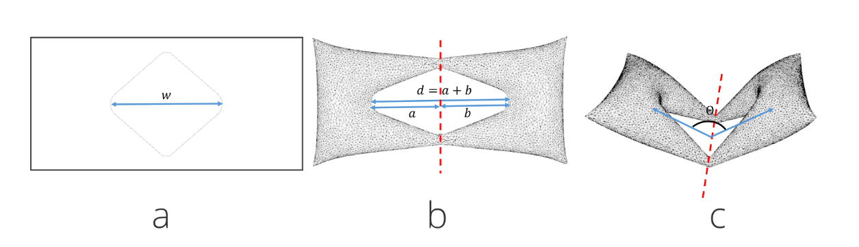
In the Aeromorph paper, the resulting angle can be derived using the law of cosines: \(\theta = \arccos\left(\frac{a^2 + b^2 - w^2}{2ab}\right)\)
Where:
- $\ a$ and $\ b$ are the lengths from the centre of the diamond to its left and right tips,
- $\ w$ is the original width of the sealed seam.
This formula gives the bending angle that preserves the seam width as the structure deforms. In this experiment, I use this setup to check whether the MeshFEM simulator reproduces that expected deformation behaviour — even though the original simulator wasn’t developed for this kind of forward geometric reasoning.
On the Scope of the MeshFEM Inflatables Pipeline
While the full simulation pipeline introduced by Panetta et al. is designed to support inverse design, generating surface seams to match a desired 3D target , my current focus lies exclusively in the forward simulation stage.
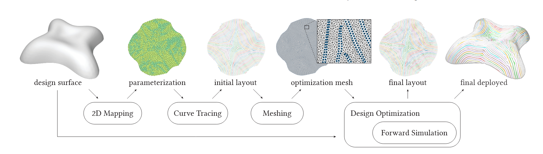
Rather than targeting a specific deployed shape, I provide predefined geometries and seam regions, and use the simulator purely to compute the resulting deformation under internal pressure.
Setup and Starting Point
The MeshFEM Inflatables repository includes a small set of Jupyter notebook examples to demonstrate usage. Since the environment is tailored for Ubuntu, I set up the simulator on a virtual machine and ran the provided demos to confirm everything was working correctly before making modifications.
Among the available notebooks, the one that served as my entry point was:
-
ForwardDesign.ipynb— a minimal forward inflation scenario based on predefined mesh and seam data
Running this notebook helped clarify the types of input files the simulator expects: primarily a .obj file defining boundary curves (no faces), along with one or more .txt files containing lists of “fused” or “hole” points.
To generate these inputs, I wrote a MATLAB script to export the required .obj and .txt files (for borders and seam masks, respectively). I then parsed them into the simulator using its forward design interface. I experimented with boundary pinning, pressure levels, and seam density to explore how much bending behaviour could be tuned using only this minimal input.
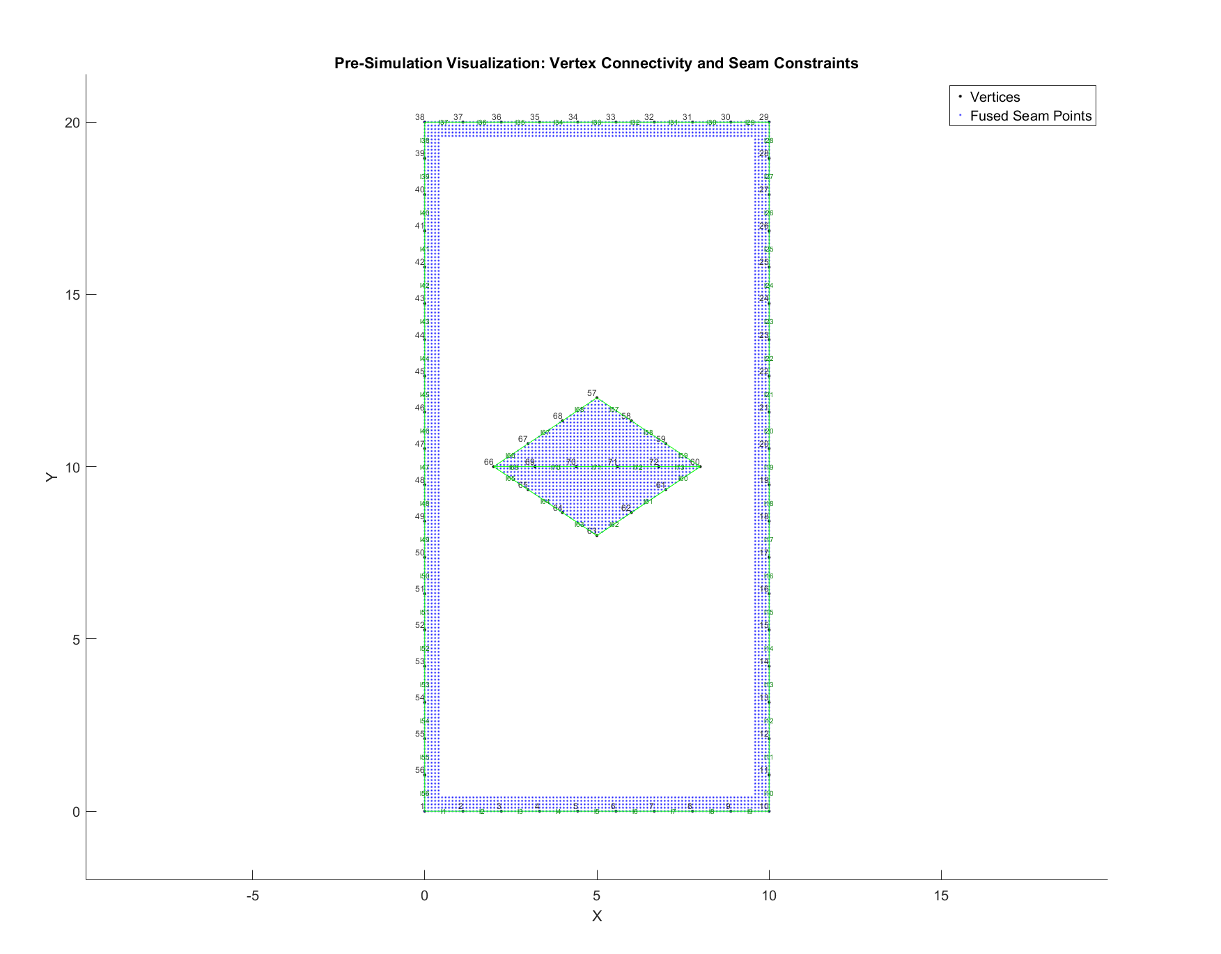
The MATLAB script I developed allows flexible specification of the input geometry. I can define an arbitrary number of vertices to outline the outer pouches and the central diamond, as well as control the density and distribution of fused points, to simulate the heat-sealed regions used in physical prototypes.
The figure below shows one of the exported configurations, with vertex labels, connected line segments, and fused seam points highlighted.
Exploring Design Variations and Their Effects
This section focuses on how I modified and tested different aspects of the input geometry and simulation setup to evaluate their influence on bending behaviour. Rather than diving into the internal workings of the simulator, I focus here on the practical effects of geometry, boundary conditions, and seam layout.
(For implementation-specific details on how MeshFEM handles meshing, region tagging, and simulation mechanics, see Inflatables MeshFEM Simulation Library)
Initial Test: Flat Inflation Without Bending
As a first test, I created the simplest layout to represent an inflatable arm, a rectangular sheet with three internal diamond shapes placed where joints would be. The idea was to mimic the typical structure of soft inflatable arms, which bend at specific hinge points along their length.
The input geometry included just the rectangle corners and the corner points of each diamond. I also placed one fused point at the centre of each diamond to represent a minimal seam. No hole regions were defined.
When I ran the simulation, the structure inflated uniformly but remained completely flat, there was no out-of-plane bending at all. The result showed that a single central seam point wasn’t enough to induce bending.
This led to a key insight: to simulate a hinge, the diamond must be divided along its horizontal axis to create two triangular regions.
From this, some design questions emerged:
- Can the direction of bending be controlled through the placement of fused points?
- Should fused points lie only along the hinge line, or also fill the surrounding area?
- How many fused points are needed to produce a noticeable bend?
After splitting the diamonds along this axis, I observed that bending did occur, but it wasn’t directional. The structure bent, but whether it bent upward or downward wasn’t predictable. This lack of control led me to simplify the geometry further to see whether seam layout could influence bending direction.
I reduced the setup to a single central diamond and tested three seam configurations:
- Fused points placed along the hinge line (the shared edge between the two triangles)
- Three fused points in a triangular pattern within each triangle, simulating a more distributed seam region
- A single fused point at the centre of the diamond (still part of the hinge line)
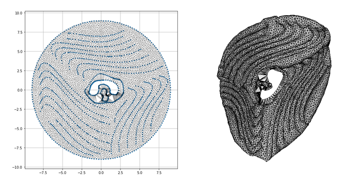
The third case — just one fused point at the centre — was sufficient to produce a clear out-of-plane bend. The mesh triangulation became asymmetric due to that single constraint, and the resulting deformation appeared to follow the direction of that asymmetry.
Simulation showing asymmetric triangulation and bending resulting from a single fused point.
At this stage, I believed that a geometric imbalance in the mesh near the seam region might be influencing the bending direction. However, this was just an early interpretation that I would later question as more tests were conducted.
Additionally, this version showed better simulation stability: there were no issues with boundary self-contact, which had occurred in earlier tests with more fused points.
Refining Geometry to Explore Bending Angle
Next, I adjusted the dimensions of the structure so that the two outer pouches (or links) would each be square, with dimensions $10×10$. This made the total sheet $10×20$, creating a simplified configuration to begin testing the geometric relationship between diamond shape and bending angle.
My goal was to explore whether modifying the shape of one triangle within the diamond would produce a bend that matched the expected outcome from the cosine rule described earlier. Although I didn’t yet get to fully asymmetric links, I expected the inflated shape to show a clear difference in bending angle. However, based on visual inspection alone, this difference wasn’t immediately obvious, which led me to start looking for a way to extract and quantify the angle without relying on perception alone.
Along the way, I also found that the final inflated mesh can be exported as a .obj file. I haven’t made use of that yet, but it could be useful later for tasks like measuring deformation, importing into other tools for analysis, or generating visual comparisons between designs.
Moving Toward Angle Extraction Through Point Tracking
At this point, I wasn’t sure how to extract any useful numerical values from the inflated geometry. But since the simulation generates the mesh dynamically and inflates it over a series of time steps, I realized I could try tracking the motion of specific points throughout the inflation cycle. By saving their positions over iteration, I could reconstruct the bend and calculate the angle based on how those points move.
This raised two immediate questions:
- Which points should I track?
- How can I reliably locate them in the actual simulation mesh?
Because the triangulated mesh is generated internally from the input curves, there’s no guarantee that a user-defined point , like the corner of the rectangle, will correspond exactly to a vertex in the final mesh. And since I had originally defined only a few key vertices (like the rectangle corners), I was concerned that none of them would align exactly with what I wanted to track.
That’s what led me to increase the number of vertices in the input geometry. By adding more points along the rectangle’s edges and interior, I improved the chances that the triangulated mesh would include nodes close enough to serve as reliable tracking anchors.
To figure out how to track motion, I first needed to choose which points to follow and how to locate them reliably in the mesh.
My initial idea was to track points along the centreline of the inflatable — for example, $[0.05,\ 0.00,\ 0.0],\ [0.05,\ 0.20,\ 0.0]$, and $[0.05, 0.40, 0.0]$. This was before scaling the model to $10×20$ dimensions, but even then the results were inconsistent. When I printed the tracked coordinates, I noticed they had shifted — possibly due to remeshing or triangulation differences between runs.
Technically, I started by locating these points in the mesh using direct distance matching against the raw vertex list (m.vertices()), but that wasn’t robust. So I switched to a more reliable method: using isheet.restWallVertexPositions() and a KDTree to find the nearest mesh vertex to each target coordinate. This made the tracking far more consistent.
To simplify, I switched to tracking along the left edge instead: $[0.00,\ 0.00,\ 0.0]$, $[0.00,\ 10,\ 0.0]$, and $[0.00,\ 20,\ 0.0]$. My reasoning was that these would be easier to identify and match across frames, and that tracking along the edge would allow me to observe the bending angle more clearly — since the deformation would occur upward or downward, it would be visible from a lateral view.
At the same time, I began thinking about fixing one of the links, as in physical setups, the base of the inflatable often rests on a surface, such as a table. In the simulation, there’s no limiting surface, so I tried pinning points along the $X-axis$ (where $Y = 0$), then by mistake on the left edge (where $X=0$),which is what the following video shows or try to create an area instead of lined point with three points like $[0, 0]$, $[0, 10]$, $[5, 10]$.
Torsion effect caused when pinning was applied along the left edge .
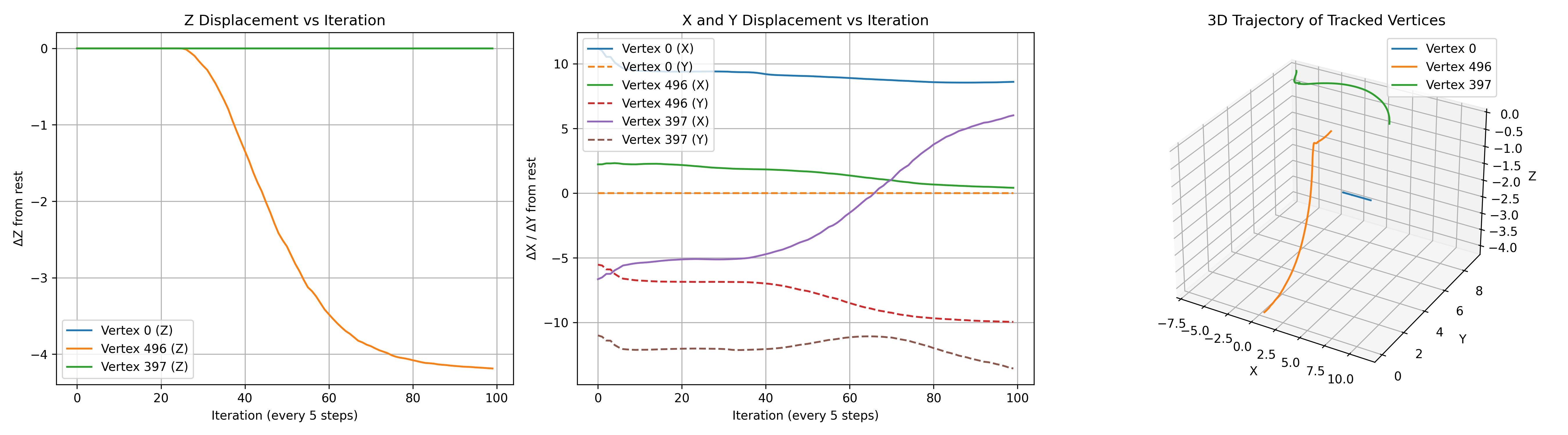
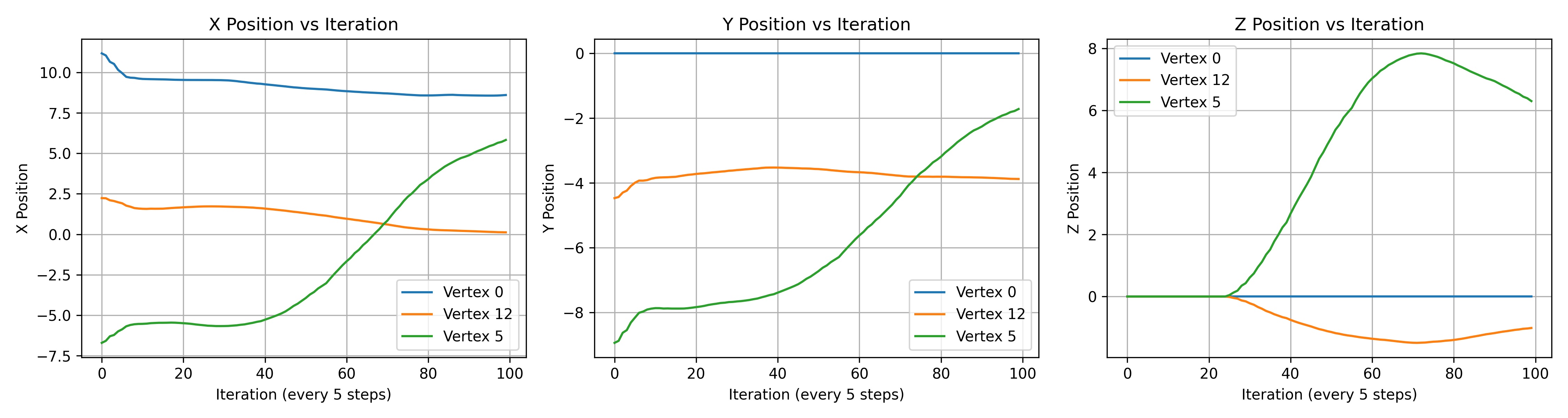
Figure 5: Plot showing the tracked positions when pinning was applied along , for the following mesh vertices: , , and . These correspond to the base, hinge, and tip along the left edge of the inflatable.
But all of these introduced unexpected torsion during inflation — a twisting behaviour that I hadn’t observed in physical tests. It’s worth noting that pinning in the simulator means constraining points in 3D space, which is different from simply resting an object on a surface under gravity.
This led me to reconsider my tracking approach. By focusing on edge points — especially on the left side — I could reduce the influence of pinning artefacts and maintain more consistent tracking across configurations.
As I revisited the various changes I’d made, I noticed something important: tracking was more stable when the tracked points were also included in the fused point list. Even with a minimal number of user-defined vertices, the meshing process reliably preserved these locations — making them easier to identify and track across frames.
Interestingly, although it’s assumed that increasing the density of fused points in a region should restrict inflation, the diamond shape didn’t appear to change visibly when I added fused points at the tracking locations. So I kept only those specific fused points — placed on the left edge (0, 0), (0, 10), (0, 20), the right edge (10, 0), (10, 10), (10, 20), and a single centre point (5, 10) at the hinge. These correspond to the base and tip of the inflatable, and the symmetric placement helped avoid introducing directional bias in the deformation.
With the pinned points removed, the simulation no longer exhibited unwanted torsion, and the results were cleaner overall.
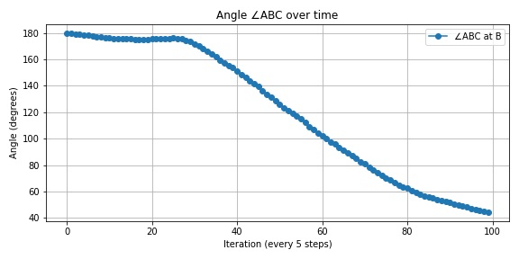
And finally, what I probably should have done from the beginning, I used the tracked points to compute the bending angle directly using the cosine rule, instead of just plotting their displacement over time.
Table: Tracked vs. Geometric Inputs
| \(\ a\) (bottom triangle height) | \(\ b\) (top triangle height) | \(Tracked\ Angle\)(simulation) | \(θ\ Calculated\) ($\ w=3$ ) |
|---|---|---|---|
| $2$ | $2$ | $44.09°$ | $97.18°$ |
| $3$ | $2$ | $50.65°$ | $70.53°$ |
| $4$ | $2$ | $100.96°$ | $46.57°$ |
Here, $\ w=3$ is taken as the seam width, based on the base length of the diamond, which remains constant across simulations.
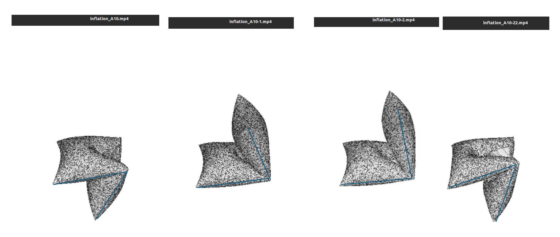
Below, I’ll include the video and plots for one of the examples (e.g. $\ a=2, b=2$) to illustrate the measurement and resulting deformation.
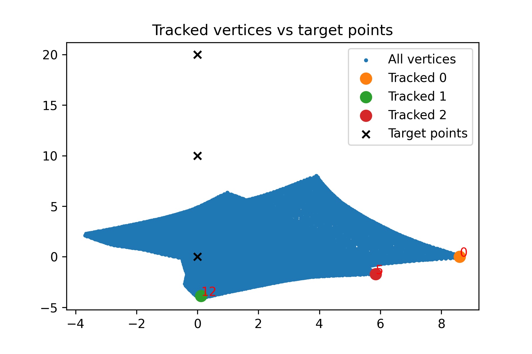
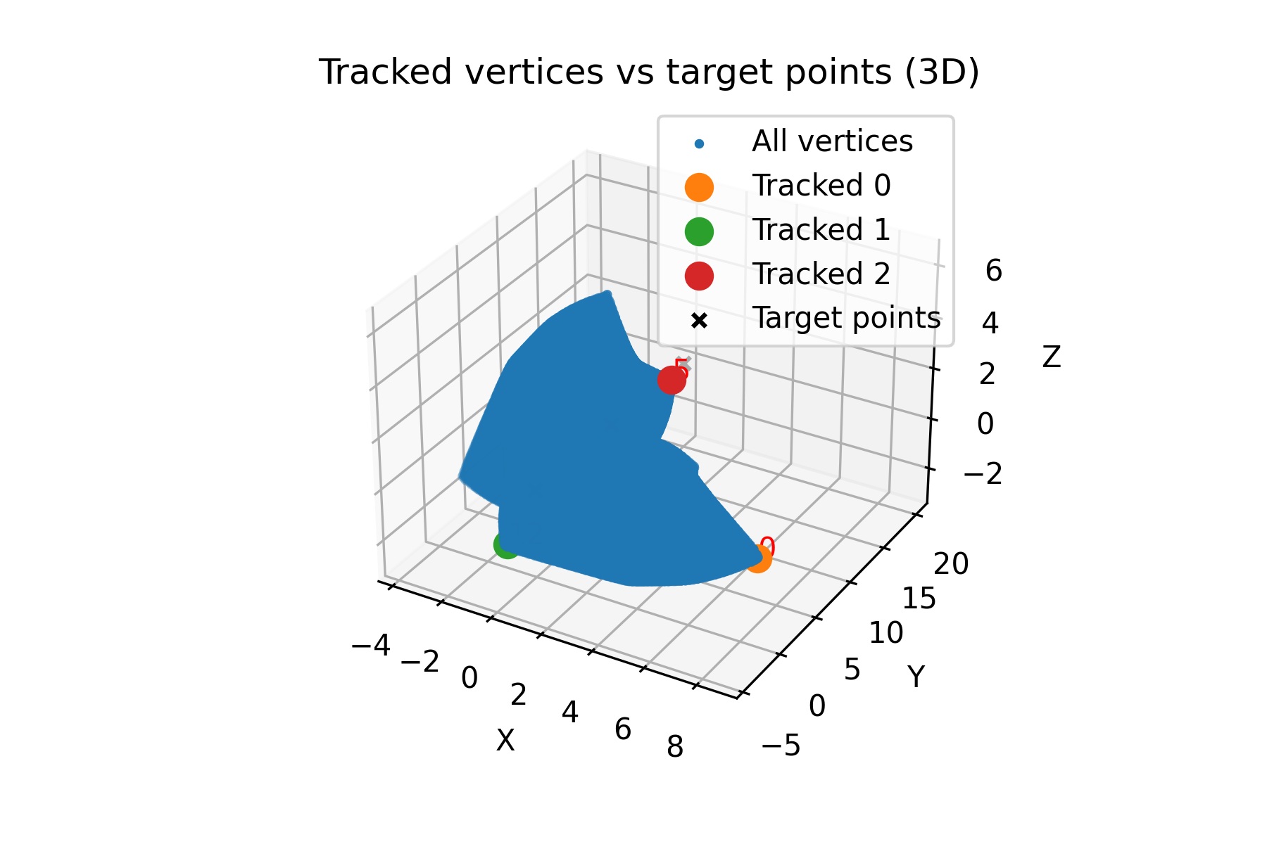
$vertex\ 0 = (0, 0)$, $vertex\ 12 = (0, 10)$, and $vertex\ 5 = (0, 20)$.
These correspond to the base, hinge, and tip along the left edge of the inflatable.
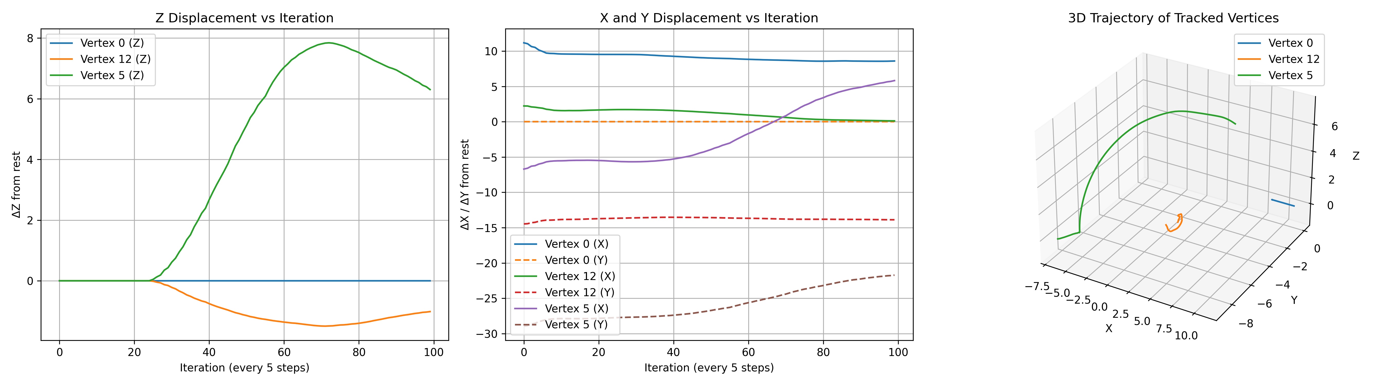
Not totally sure how much these add beyond curiosity value, but they were a way to check where the tracked points ended up compared to their intended targets. The 2D version flattens everything so it can be a bit misleading, while the 3D view gives a clearer sense of how far they’ve moved in space.
On Formula Discrepancy
The bending angle formula used earlier,
\[\theta = \arccos\left(\frac{a^2 + b^2 - w^2}{2ab}\right)\]assumes a specific geometric interpretation: $a$ and $b$ are the lengths from the hinge point (where the two triangles meet) to the seam tips, and $w$ is the seam width — the inextensible distance between those seam tips.
However, in some diagrams (like Figure 1 from the Inflatables paper), $a$ and $b$ are shown as horizontal components, implying that $w = a + b$. If we plug this into the equation:
\[\theta = \arccos\left(\frac{a^2 + b^2 - (a + b)^2}{2ab}\right) = \arccos(-1) = 180^\circ\]we get a flat structure with no bending, which contradicts both the physical outcome and the aim of the formula. This highlights a key misunderstanding: if $w = a + b$, the equation will always yield $180°$, meaning no bending occurs. So, for bending to happen, $w$ must be strictly less than $a + b$.
This mismatch between diagram labelling and formula assumptions likely contributes to the discrepancy between simulated angles and theoretical predictions.
I plan to revisit the exact relation between the physical geometry, seam layout, and the angle prediction formula.
Physical Reference: Aeromorph Hinge Behaviour
The Aeromorph paper provides a physical reference, showing that as the height of the diamond increases (while width is fixed), the resulting bend becomes more pronounced.
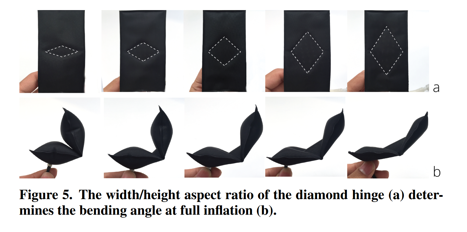
In my case, I varied $a$ while keeping $b$ fixed as a way to control the triangle proportions and induce different bending angles under the law of cosines. However, based on the diagram discrepancy and physical results, I will revisit the mapping between design parameters and analytical predictions to ensure the setup reflects the intended formulation.
Notes mentioning this note
There are no notes linking to this note.